Usage

This section provides an overview of how to use the ‘deeplogs’ library.

Setup & Imports

Import the library.

import deeplogs as dpl

You can define a dictionary that contains the configuration of your model.

model_hyperparam = {
    "version": 4,
    "epoch": 1,
    "batch_size": 128,
    "lr": 1e-3,

    "x_shape": (512,512),
    "y_shape": (10,),
    "nb_layers": 8,
}

The Logger here takes in three arguments:

a string containing a run name
a description of the run
and the configuration dictionary created earlier

logger = dpl.Logger(
    "v" + str(model_hyperparam["version"]),
    "A description of the run",
    model_hyperparam,
)

Implementation

In this illustrative code, model performance is generated randomly, and the outcomes are meticulously logged.
During each epoch and batch iteration, the “logs” dictionary is continuously updated with important metrics such as “acc”, “loss”, “val_acc”, and “val_loss”.
These results are subsequently saved using the ‘logger.scalar()’ method. Finally, we use the flush method to save the latest logs immediately.

model_perf = random()
for epoch in range(model_hyperparam["epoch"]):
    size = 1000
    for batch in dpl.Bar(logger, f"Epoch {epoch+1}")(range(size)):
        logs = {}

        logs["acc"] = log(batch+1) * model_perf
        logs["loss"] = size/exp((batch+1)/size) * model_perf
        logs["val_acc"] = log(batch+1) * model_perf
        logs["val_loss"] = size/exp((batch+1)/size) * model_perf

        timestep = epoch + (batch/size)
        logger.scalar(timestep, **logs)

        sleep(0.005)
logger.flush()

>>> Epoch 1: 100%|██████████| 1000/1000 [0:00:05<0:00:00, 196.82it/s] acc: 1.761 | loss: 93.771 | val_acc: 1.761 | val_loss: 93.7711

That’s all you need to integrate into your model’s learning loop to get data and monitor your model.

Results

Scalars

Create the reader

reader = dpl.Reader()

Display information about the runs.

reader.infos()

name	description	version	epoch	batch_size	lr	x_shape	y_shape	nb_layers
v1	A description of the run	1	1	128	0.001	(512, 512)	(10,)	8
v2	A description of the run	2	1	128	0.001	(512, 512)	(10,)	8

Display a summary of the metrics used during the training of your model.

reader.describe()

name	description	acc	loss	val_acc	val_loss
v4	count	5000.000000	5000.000000	5000.000000	5000.000000
	mean	1.950368	208.427719	1.950368	208.427719
	std	1.308797	151.283633	1.308797	151.283633
	min	0.000000	40.007505	0.000000	40.007505
	25%	0.741063	81.293497	0.741063	81.293497
	50%	1.568038	154.525183	1.568038	154.525183
	75%	3.333099	308.287299	3.333099	308.287299
	90%	3.908165	448.516692	3.908165	448.516692
	max	4.343923	628.218730	4.343923	628.218730

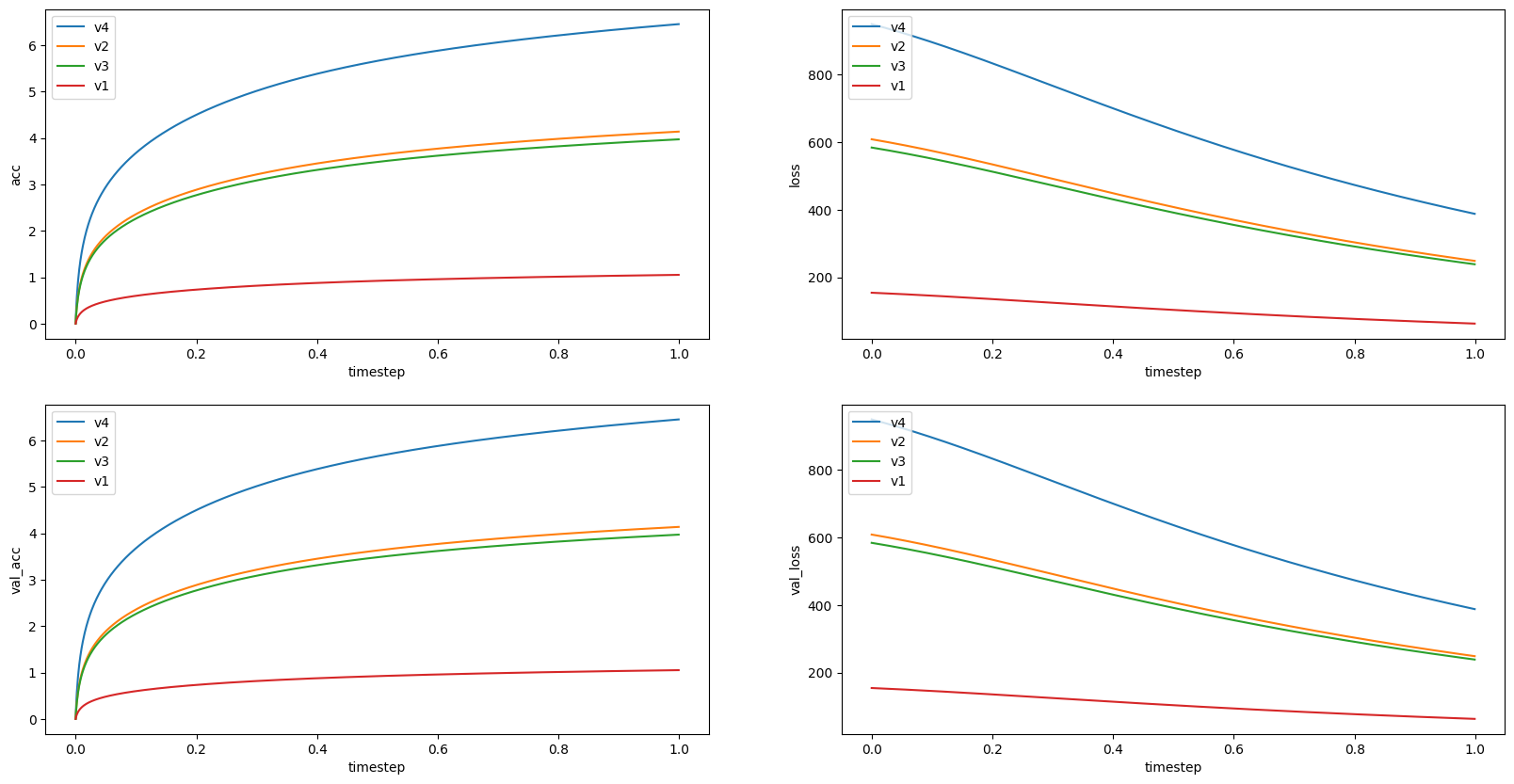
Display scalar data using Matplotlib.

reader.scalar(using="matplotlib")

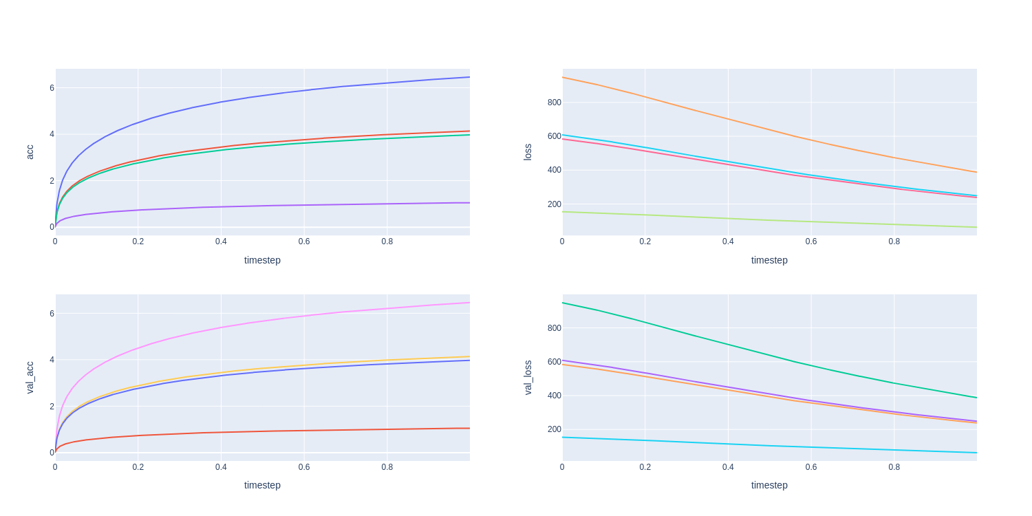
Display scalar data using Plotly.

reader.scalar(using="plotly")

Images

To demonstrate image handling, we start by opening an example image and converting it into a NumPy array.

img = np.asarray(Image.open("../assets/logo.png"))[:,:,:3] / 255
fig = plt.imshow(img)

Next, we perform various transformations on the image to explore its dimensions and formats.

img1 = img
img2 = img.transpose(2,0,1)
img3 = img.transpose(2,0,1)[None].repeat(16,0)
img4 = img.transpose(2,0,1)[None].repeat(128,0)
img5 = img[:,:,0]

For the original image, the dimensions are (height, width, color), i.e., (500, 500, 3).

>>> img1.shape (500, 500, 3) # (height, width, color)

o log this image, the “HWC” format should be used.

logger.image(12, img1, "image1", "HWC")

>>> img2.shape (3, 500, 500) # (color, height, width)

logger.image(1, img2, "image2", "CHW")

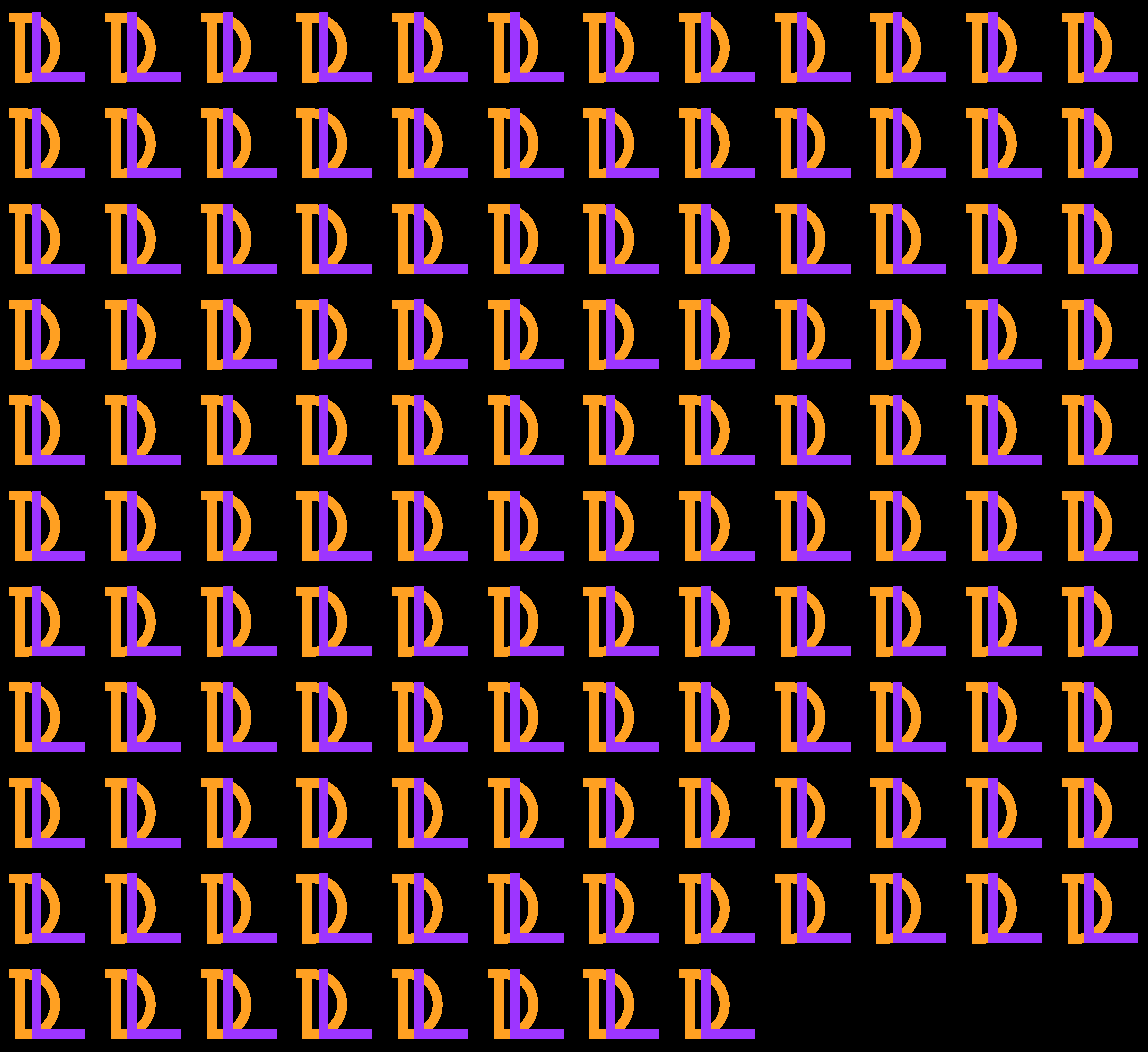
When multiple images are provided in a batch, the method creates a single grid-like image.

>>> img3.shape (16, 3, 500, 500) # (batch, color, height, width)

logger.image(0.001, img3, "image3", "NCHW")

To log this batched image, the “NCHW” format is required.

>>> img4.shape (128, 3, 500, 500) # (batch, color, height, width)

logger.image(0.9, img4, "image4", "NCHW")

Even if the image has no color dimension, the method saves the image as grayscale with dimensions (height, width), i.e., (500, 500)

>>> img5.shape (500, 500) # (height, width)

logger.image(0., img5, "image5", "HW")